THERMO Spoken Here! ~ J. Pohl ©

TOC NEXT ~ 41

Blue Ocean Towing

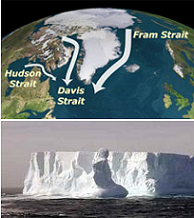
Davis Strait passes between Baffin 
Island and Greenland. It was explored
by John Davis in 1585.

Our company is contracted to protect an ocean oil rig situated in Davis Strait. A massive slab of ice, ( ~ 800x10⁶kg) having cleaved from the ice-shelf, is drifting by sea current directly toward the rig. Cables will be attached to the slab whereupon pulling steadily (at 90° to the current) our tugs will drag the slab off-course to pass abreast the rig no closer than 4000 meters. There is time to do this, provided our tugs, in unison, are up to task.

Calculate the constant towing force our tugs must sustain to accomplish the task. Use the information provided with assumptions as required.

Nautical situation at the
commencement of tow.

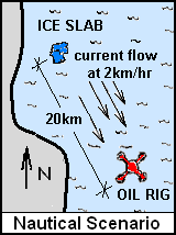
♦ As system, we model the ice slab as a BODY. A towing cable will extend from the slab to the tugs. At an arbitrary place, a distance from the slab, imagine our system boundary to pass through, to cut through the cable. The "towing force" will act over the face of the imaginary cut of the cable. The sketch, Nautical Scenario, shows the initial location of the slab relative to the the production rig.

Since the slab will not move in a vertical direction, we set our coordinate reference to be an 0XY plane-of-motion,coordinates x and y, with unit vectors I and J. See sketch Coordinates and Basis below.

We will use Momentum analysis, Newton's Second Law, as written below, Eqn-1, to attempt a solution.

(1)

It is wise to express time-dependent terms explicitly by
attaching “(t)”. 
For example, better to write V(t) than simply V. 

Drag forces are expressed discretely and vary over parts of the 
system surface.  Hence those forces are rightly preceded by the Greek
sign, sigma (Σ). Meaning: drag forces require 
careful summation.

Most students at this level of study are familiar with Newton's Second Law written in its simplest, algebraic form as f = ma. Eqn-1 is Newton's Second Law written in vector form as a statement of conservation of momentum. Forces are the causes of momentum change. Perhaps re-read About: f = ma to review the connection. Also students are minimally aware of drag forces which are represented in the equation statement.

We visualize the slab to drift with the constant-speed current toward the rig. Drag forces occur over system surfaces (at all locations of system/surrounding boundaries) where there are system to surrounding relative-velocity-differences. At all locations of motion of the system boundary, matter of the surroundings opposes that motion. Surroundings of this slab are sea water, atmospheric air, and the average force acting over the area of "cut" across the cable. Most of slab surface is submerged having ice-to-seawater contact. The slab upper surface has ice-to-atmosphere contact.

At this level we cannot write expressions for drag. We know the forces are proportional th relative speed squared. The slab moves quite slow, so we assume the drag to be sufficiently small as to be neglected and struck, " / " from Eqn-1. To proceed we must do this.

The next step is to expand the derivative of momentum of the slab; expand the term left of equality.

(2) Movement of the slab through the sea and air above is opposed by the sea and air. These resistive effects are called "drag forces." Since the slab velocity will be very small, we assume drag forces of the event to be negligibly small.

Slab Mass might change during the event as some of it melts into the sea. To assume melting to be small is equivalent to assuming the mass of the slab to be constant. To apply this idea we expand the derivative, d(m(t)V(t))/dt, and set (dm(t)/dt)V(t) ~ 0.

The notation, single slash, / , drawn through an equation term means the term is neglected because:
i) It is known to be small (but not zero) or,
ii) To include the term makes the solution prohibitively difficult.
Consequently the term is set to zero and an approximate solution
is sought.

Thus our momentum equation becomes Eqn-3:

(3)

This first order, vector, differential equation describes
the relation of forces and motion of the slab.  The dependent
variable is the "velocity" of the slab, V(t). The independent 
variable is time, "t."  Mathematics calls the term, 
F(t),  non-homogeneous.

Eqn-3, a first-order, vector, ordinary differential equation, is solved by its integration. Steps prior to integration are: i) separation of variables, ii) application of the integral operator, then iii) specification of the integral limits. The notations are known by now; we omit those details hereafter.

i) The dependent variables are slab velocity, V(t) and the tow force F_tow(t). The independent variable is time, t. Simply multiplty Eqn-3 by "dt," it becomes "separated." Eqn-4 results:

(4)

This differential equation is in its "separated" form.
We see to "separate variables" amounts to a simple 
multiplication of Eqn-5 by dt. That is all there 
is to it.

Now apply the linear operator for integration ( ∫ ) to Eqn-4. Mass is constant, it is moved ahead of the symbol. With this step we "indicate" the limits of the integrals (to be entered soon). "u.l." means upper limit and so on.

(5)(5)

We chose coordinates, X and Y, conveniently.
Our vector basis will be I and J. The sketch
shows the initial position and the “intended”
final position of the slab. The manipulations (Eqn-1 through Eqn-5) were mostly qualitative. To proceed, to specify limits, a moreso quantitative approch is needed. A working sketch and a table are needed.

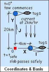
Our previous sketch is modified to include an origin, coordinate system and vector basis. In Coordinates & Basis, an origin of an OXY-plane is placed at the oil rig. A Y-axis is directed toward the initial position of the slab, with an X-axis perpendicular to the Y-axis. Unit vectors I and J are assigned as shown.

Shown also is the position of the slab at commencement of tow, when the time is: t = 0⁺. The second time of importance is not known but the location of the slab is known. We label the second time as t = t_safe. The brief table shows relevant times, positions and velocities of the event.

	Instant	Position	Velocity
Start:	t = 0+	P = 20,000mJ	V = 2km/hr (-J)
Safe:	t = t_safe	P = 4000m I	V = v_xI + 2km/hr (-J)

The table serves us to specify limits for the integrals. Limits for the integral right-of-equality, having the differential, "dt," are usually easier limits to specify. The initial condition for the independent variable, time, is the initiation of the tow. We have designated that initial time as, t = 0+. (In effect, we take the event to be an epoch). The upper limit we specify (for now) as some "indefinite" later time. The upper limit is written, t.

Upper and lower limits of the integral left-of-equality correspond physically with those of the integral of "dt" (right-of-equality). Thus the lower limit of the integral left-of-equality, having the differential "dV," must be the velocity of the slab at time, t = 0+. The slab at that time is drifting with a velocity equal to that of the sea current: V_{slab, t = 0+} = (2 km/hr)(-J). The negative sign associates with the direction part of the velocity, not its magnitude.

(6)

The equation, with limits of both integrals 
applied, is ready to be integrated.

In the above equation, the integral left-of-equality has "1" as its integrand. This integral is said to be "exact." It integrates immediately to be the difference: upper limit minus lower limit. The equation with "left-of-equality" integrated is written below - Eqn-7.

(7)

Left-of-equality integrates immediately. The integral 
right-of-equality requires more information.

The right-side-integration implies the magnitude of the towing force might vary over the durration of towing in any number of ways. Put otherwise, there is no single solution for "towing force" that will get the job done. The extra information needed is that the tow force is constant and it acts 90° to the drift.

(8) The Mean Value Theorem (MVT) will transform the integral right-of-equality
to the average force times the duration of its action.

The integration above yields the velocity of the slab. The constant tow force cannot be obtained. to proceed, we are use the fact, V(t), equals dP(t)/dt. We make that substitution and to move on, we separate variables and apply limits in the same style as before. Please do the algebra to confirm the correctness of the following equation:

(9) A number of steps were required to arrive here.
Please check the changes.

The limits of the integral left-of-equality are vector positions. The slab is initially directly upstream of the rig a distance of 20,000 m. The rig is at the origin hence the lower limit of the integral is 20,000 m J. The final or safe position of the slab is 400 meters directly abreast of the rig. The lower limit is 400 m I. Also, the integrand ahead of dP is "1." The integration of an exact differential equals its "upper limit minus lower limit." Right of equality we have an integral of "t dt" and one of "dt." The changes for all terms yield...

(10) Next we use the fact that the component equations of a vector
equation are independent. To obtain the component equations we
multiply this vector equation by J to obtain one component equation
then by I to obtain the second equation. These equations are independent.

Above we clearly see an equation with an "I" component and a "J" component. The fancy way to get two independent equations from this vector equation is to use vector scalar multiplication. The equation, scalar multiplied by the unit vector, J provides important information:

(11)

The J - component equation tells
us the duration of tow is 10 hours.

The J component states that the time of the event will be 10 hours. When Eqn-11 is multiplied by the unit vector, I, the following expression is obtained:

(12) This "I - component equation, results from scalar multiplication of Eqn-14 by
the unit vector, I.

The duration of the event is known. It can be entered into the above equation to yield a solution for the Average Towing Force.

(13) The I - component when combined with the result of the J - component
yields the average value of the towing force required of the tug.

The answer as to the force the towing cable must withstand is quite approximate. Its greatest value might be that we have no other number. The nature of any assumption is to return a "rosy" answer. Our calculations do not tell us how strong the towing line must be. Our calculations tell us that any line with a strength less than our answer will fail.